Movable Type

Prologue

Books are fun. ^{[citation needed]}

What’s even more fun are vector space models, clustering algorithms, and dimensionality reduction techniques. In this post, we’re going to combine it all and play around with a small set of texts from project Gutenberg. With a bit of luck (and lots of Python) we might just learn something interesting.

Chapter One: Index Librorum

First, we’re going to need some books. Let’s be lazy about it and just use what NLTK has to offer:

from nltk.corpus import gutenberg

fileids = gutenberg.fileids()
print(', '.join(fileids))

austen-emma.txt, austen-persuasion.txt, austen-sense.txt, bible-kjv.txt, blake-poems.txt, bryant-stories.txt, burgess-busterbrown.txt, carroll-alice.txt, chesterton-ball.txt, chesterton-brown.txt, chesterton-thursday.txt, edgeworth-parents.txt, melville-moby_dick.txt, milton-paradise.txt, shakespeare-caesar.txt, shakespeare-hamlet.txt, shakespeare-macbeth.txt, whitman-leaves.txt

This rather eclectic collection will serve as our dataset. We can weed out some boring books and fetch the full texts for the rest. Let’s also be pedantic and format the titles:

import re

boring = {'bible-kjv.txt',
          'edgeworth-parents.txt',
          'melville-moby_dick.txt'}

fileids = [f for f in fileids if f not in boring]
books = [gutenberg.raw(f) for f in fileids]
titles = [t.replace('.txt', '') for t in titles]

Conveniently, and completely coincidentally, the remaining titles fall roughly into five categories I spent far too much time naming:

• Novel and Novelty: Emma, Persuasion, Sense and Sensibility

• Bard’s Tales: Julius Caesar, Hamlet, The Scottish Play¹

• Chestertomes: The Ball and the Cross, The Wisdom of Father Brown, The Man Who Was Thursday

• BBC (Bryant, Burgess, Carroll): Stories, The Adventures of Buster Bear, Alice’s Adventures in Wonderland

• BMW (Blake, Milton, Whitman): Poems, Paradise Lost, Leaves of Grass

In other words, our modest library contains three Jane Austen’s novels, three Shakespeare’s plays, three novels by Gilbert K. Chesterton, three children books (I’m sorry, Mr Carroll) and some poetry. Let’s see if that classification is equally obvious to a machine.

Chapter Two: A is for Aardvark

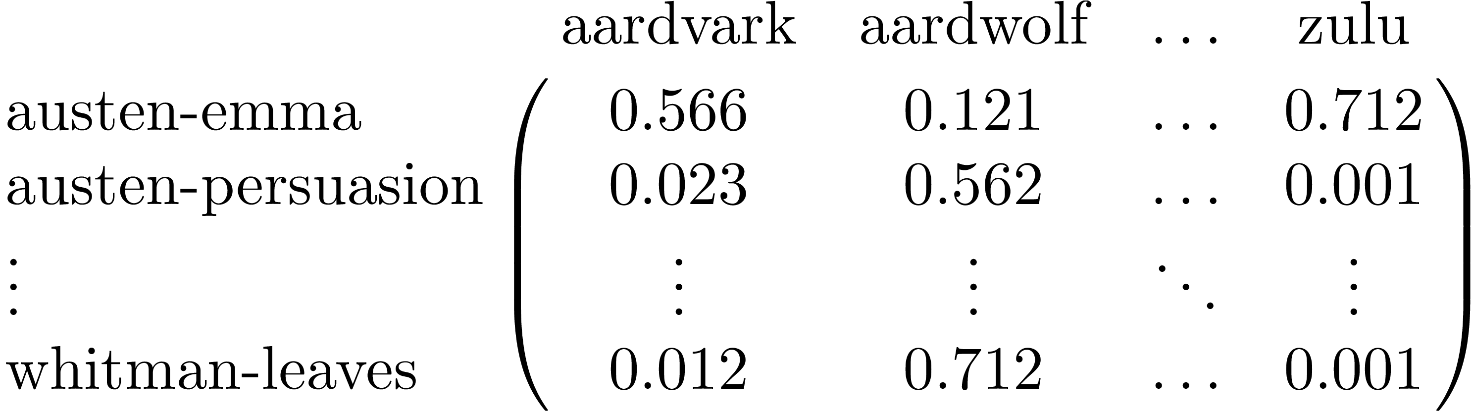
Computers are basically illiterate, but they’re pretty good with numbers. That is why we need to represent the books as numerical vectors. We’re going to use term frequency-inverse document frequency (tf-idf). Technical details aside, words with highest tf-idf weights in each book will be those that occur a lot in that book, but don’t occur in many other books. Once we calculate the tf-idf weights, we can build a matrix with columns corresponding to terms and rows representing books:

To avoid reinventing the wheel, we’ll ask scikit-learn to do all² the work. It can even filter stop words, normalize term vectors and impose constraints on document frequency (max_df=.5 means we ignore terms that occur in more than half of the books):

from sklearn.feature_extraction.text import TfidfVectorizer

vectorizer = TfidfVectorizer(max_df=.5, 
                             stop_words='english')

tfidf_matrix = vectorizer.fit_transform(books)

The result is a (sparse) numerical matrix, so we need to find out which row/column corresponds to which book/term. The order of rows is the same as in books, so that part is easy. Getting the list of terms is a bit more tricky:

terms = vectorizer.get_feature_names()

The terms are sorted alphabetically, so the beginning of the list will be mostly numbers. Here’s a slightly hacky way to see some words:

a = [t for t in terms if t.startswith('a')][:5]
z = [t for t in terms if t.startswith('z')][-5:]
print(' '.join(a))
print(' '.join(z))

aaron aback abandon abandoned abandoning
zoological zophiel zso zumpt zuyder

Cool! No aardvarks or aardwolves, but at least Aaron is there. We can now find top terms for each book by argsorting the book vectors:

top_indices = (-tfidf_matrix).toarray().argsort()[:, :5]

for index, title in enumerate(titles):
    top_terms = [terms[t] for t in top_indices[index]]
    print(f"{title}:\n{' '.join(top_terms)}\n\n")

austen-emma: 
emma harriet weston knightley elton

austen-persuasion:
anne elliot wentworth captain charles

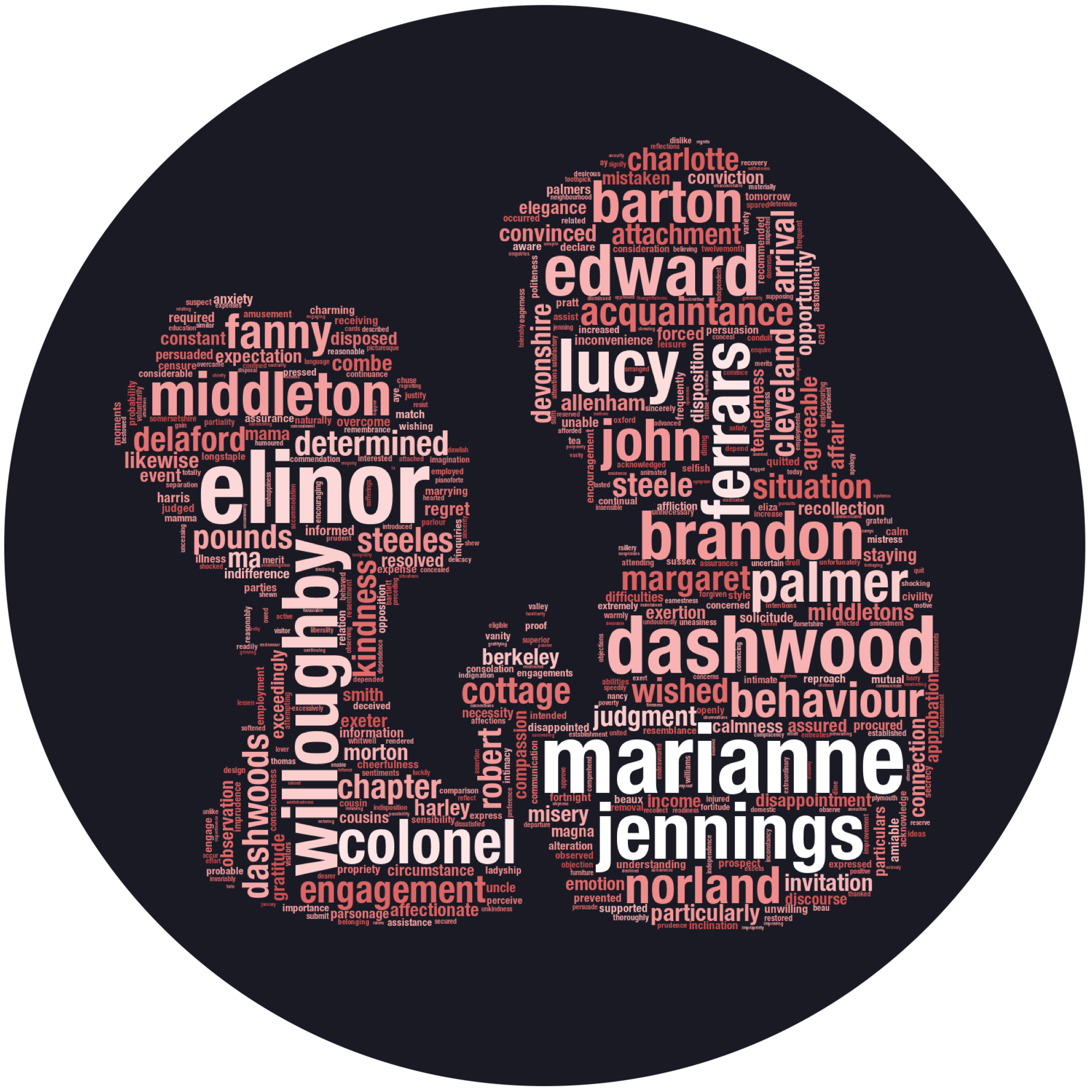
austen-sense:
elinor marianne dashwood jennings willoughby

blake-poems:
weep thel infant lamb lyca

bryant-stories:
jackal margery nightingale big brahmin

burgess-busterbrown:
buster joe farmer blacky sammy

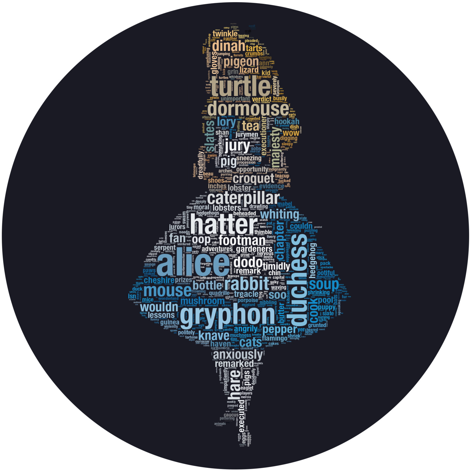
carroll-alice:
alice gryphon turtle hatter duchess

chesterton-ball:
turnbull macian evan police gutenberg

chesterton-brown:
flambeau muscari boulnois fanshaw duke

chesterton-thursday:
syme professor gregory marquis bull

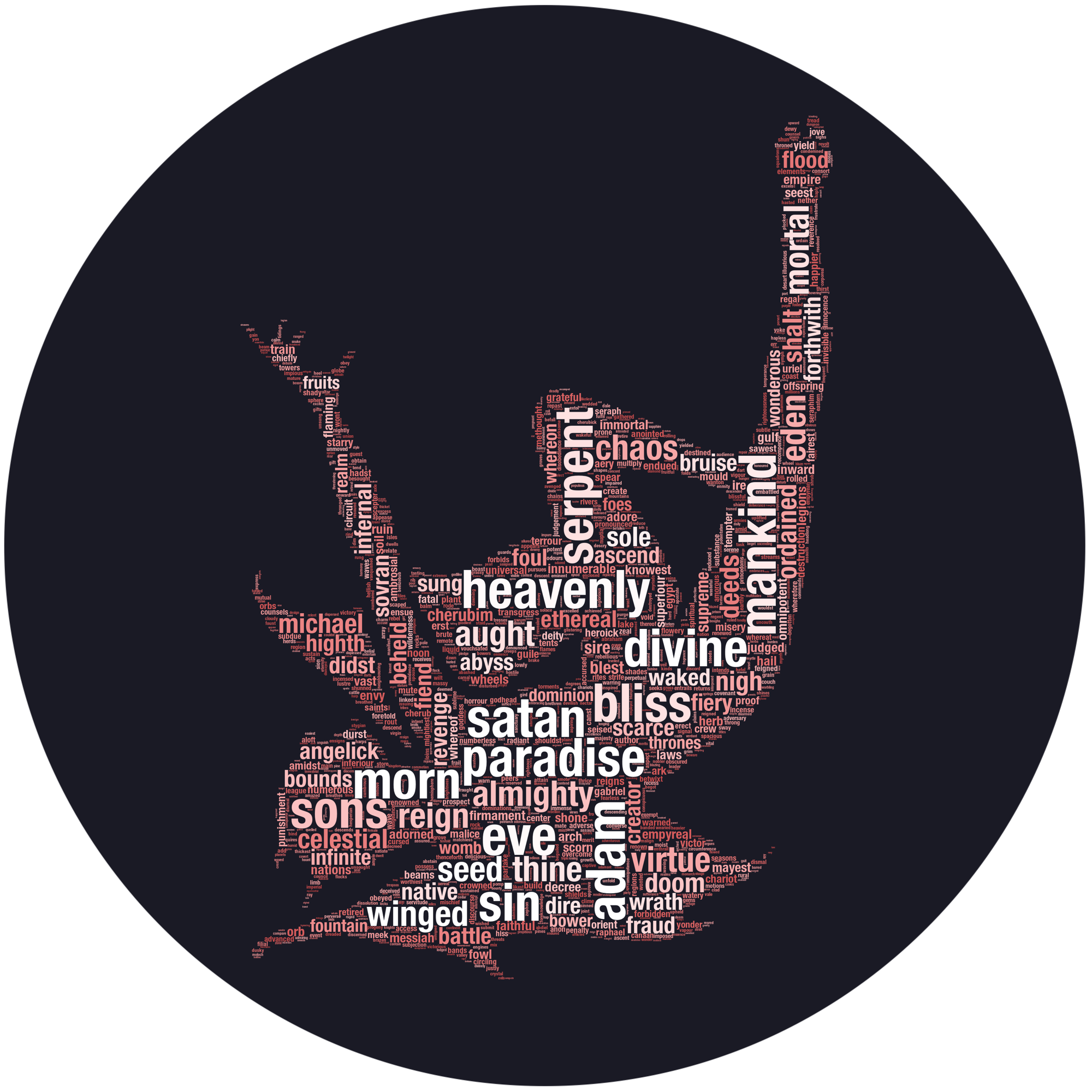
milton-paradise:
hath adam eve satan spake

shakespeare-caesar:
brutus cassius caesar haue antony

shakespeare-hamlet:
hamlet haue horatio queene laertes

shakespeare-macbeth:
macbeth haue macduff rosse vpon

whitman-leaves:
states poems cities america chant

Our library is rather small, so dull words like spoke and had unfortunately made the cut, just because Milton and Shakespeare spelled them funny. This could be fixed by adding all the haues, spakes, vpons, and haths to the stop word list. Apart from that, the results are pretty informative, with character names generally scoring highest on tf-idf.

Curiously, it seems Brutus stole the show from the eponymous character of Shakespeare’s Julius Caesar (et tu, Brute?) and Satan is more prominent than God in Paradise Lost. The latter case is particularly interesting, as it sheds some light on how tf-idf works. A quick grep shows that 327 verses of Milton’s poem take the Lord’s name in vain, while only 72 feature Satan, so good triumphs over evil as far as term frequency is concerned. However, Satan is mentioned less often in other books in our collection, so (s)he³ scores much higher on inverse document frequency.

Lyric poetry features fewer characters, so only Blake’s Lyca and Thel make it to the top five. Instead, we get an insight into poets’ favourite topics – it appears Whitman was really into America, while Blake’s work involve lots of weeping lambs.

Chapter Three: Wordcloud Atlas

For a more artistic take, let’s visualize the tf-idf vectors using the wordcloud module. I’ll let you guess which is which.

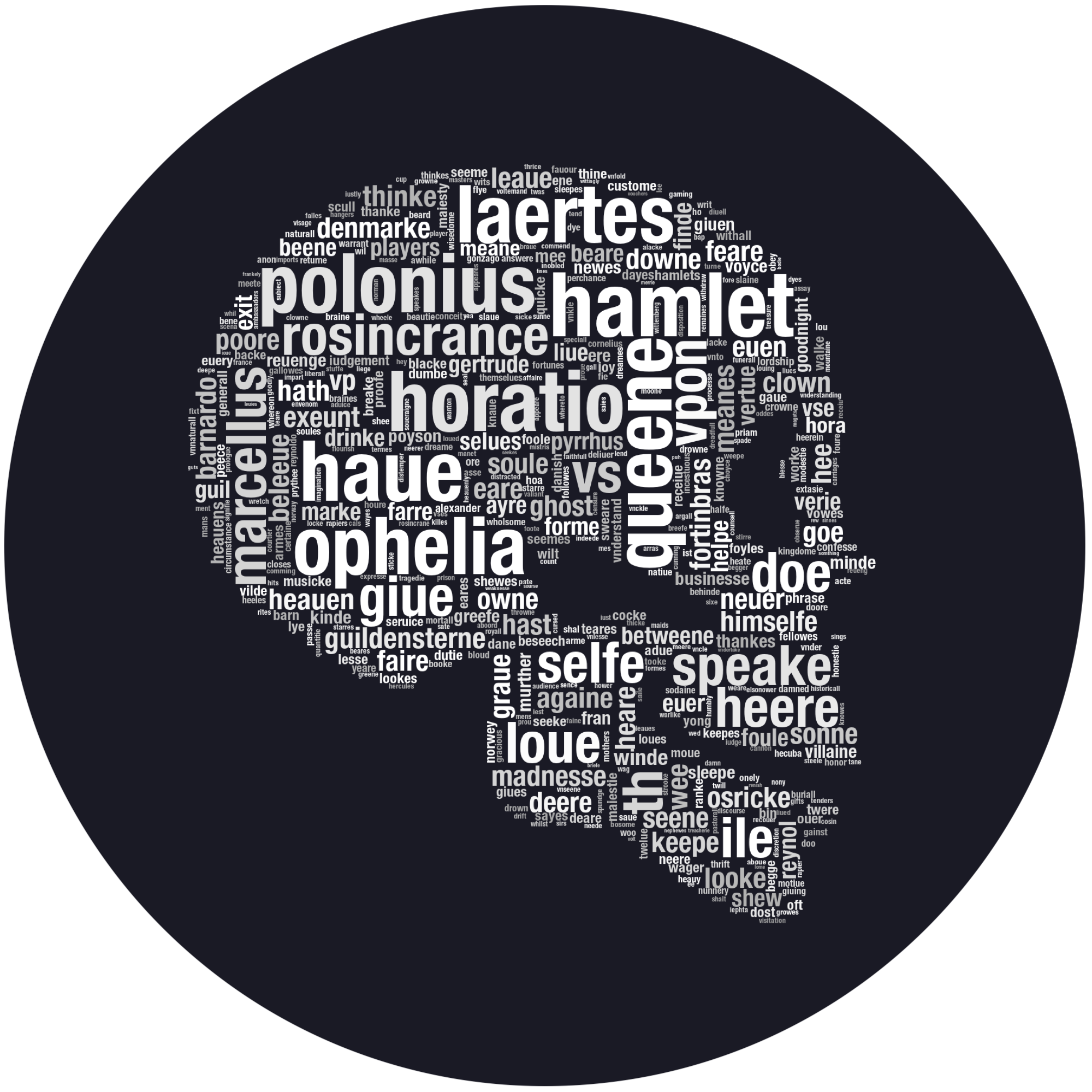
Poor Yorick tells us quite a lot about Shakespearean orthography. It seems y was often used in place of i (voyce, poyson, lye) and u/v could represent either a vowel or a consonant, with v used at the beginning (vpon, haue, vs). Moreovere, it woulde seeme silente finale ees were quite populare.

Chapter Four: k-Means to an End

Wordclouds were a cool digression, but it’s time to get back to the main question – what happens if we try to automatically group our books into categories? We’ll use the k-means clustering algorithm to find out. To understand how it works, think of every book vector as a point in a high-dimensional space. We start by randomly choosing k points as means, create clusters by assigning every book to the nearest mean and then move each mean to the center of its cluster. After repeating this process a couple of times, it usually converges, although often to a local optimum. How do we choose k? We can just set it to five, since we want five clusters, but in general it’s a problem deserving at least a Wikipedia page.

Once again, sklearn has us covered – it even works on sparse matrices! We can find the clusters in two lines of code (and then spend six more trying to print them):

from sklearn.cluster import KMeans
from collections import defaultdict

kmeans = KMeans(n_clusters=5)
labels = kmeans.fit_predict(tfidf_matrix)

clustering = defaultdict(list)
for title, label in zip(titles, labels):
    clustering[label].append(title)
    
for cluster, elements in sorted(clustering.items()):
    print(f"Cluster {label}: {', '.join(elements)}")

0: bryant-stories, burgess-busterbrown
1: austen-emma, austen-persuasion, austen-sense, chesterton-ball, chesterton-brown, chesterton-thursday
2: shakespeare-caesar, shakespeare-hamlet, shakespeare-macbeth
3: blake-poems, milton-paradise, whitman-leaves
4: carroll-alice

Not bad! First of all, I owe Mr Dogdson another apology. Alice is in a class of its own and doesn’t belong with children stories. Instead, Jane and G.K. have to share a cluster. The rest is as expected – poets stick together⁴ and Shakespeare’s tragedies are in one place. When I ran it with n_clusters=6, Chesterton and Austen got a room of their own, but Alice was still lonely.

If you run it a couple of times, you might notice you’re getting different outcomes. This is the local optimum problem. We can try to avoid it by running the algorithm multiple times and choosing the best result. Actually, this already happens behind the scenes: by default, sklearn returns the best of 10 runs. Unfortunately, we can still get unlucky and hit a sub-optimal solution every time. Let’s run it 50 times and see if anything changes:

kmeans = KMeans(n_clusters=5, n_init=50)

0: blake-poems, milton-paradise, whitman-leaves
1: austen-emma, austen-persuasion, austen-sense
2: chesterton-ball, chesterton-brown, chesterton-thursday
3: shakespeare-caesar, shakespeare-hamlet, shakespeare-macbeth
4: bryant-stories, burgess-busterbrown, carroll-alice

Nice! This time we find a better solution and the clustering is exactly as expected. Unless you’re really unlucky, the result should be consistent if you re-run the code. But how do we know it’s better? The k-means algorithm chooses a solution with lowest inertia. We can use it to compare different clusterings:

print(kmeans.inertia_)

8.985937270983072

Inertia is the sum of squared Euclidean distances⁵ of cluster elements to their closest mean. Minimizing it is a good idea in our case, because we expect a known number of similar-sized, well-separated, convex clusters. The world is rarely so perfect, so good clustering means different things in different contexts.

Chapter Five: A Romance of Many Dimensions

The final step is to find a way to visualize the clusters. There is just one small problem, and it’s a big one: book vectors live in a really-high-dimensional space:

print(len(terms))

28282

People generally have trouble visualizing more than three dimensions⁶. We’ll use principal component analysis to find a human-friendly, two-dimensional representation of our data:

from sklearn.decomposition import PCA

dense_tfidf_matrix = tfidf_matrix.todense()
pca = PCA(n_components=2)
points_pca = sklearn_pca.fit_transform(dense_tfidf_matrix)

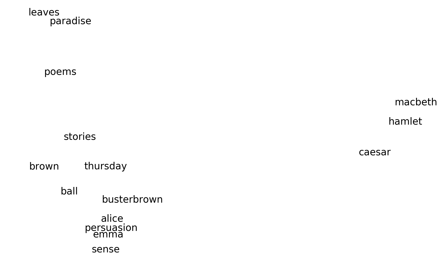
The result highlights the difference between poetry, prose, and drama, but the three clusters within prose are all mingled. Still, it’s pretty impressive considering we’re essentially projecting 28282 dimensions on a plane.

Anyway, PCA is so 1901 and all the cool kids are using t-SNE now. It works just like magic – it’s powerful, hard to understand, and easy to abuse. The algorithm has three knobs: perplexity, learning rate, and the numbers of iterations. However, their effect on results might be hard to figure out:

If you’d like some intuition about how it works, this article offers a detailed look inside the black box. The important rule of thumb is that t-SNE will freak out if perplexity is greater than the number of points. I used the following configuration:

from sklearn.manifold import TSNE

tsne = TSNE(n_components=2,
            learning_rate=10,
            perplexity=10,
            n_iter=500)
points_tsne = tsne.fit_transform(dense_tfidf_matrix)

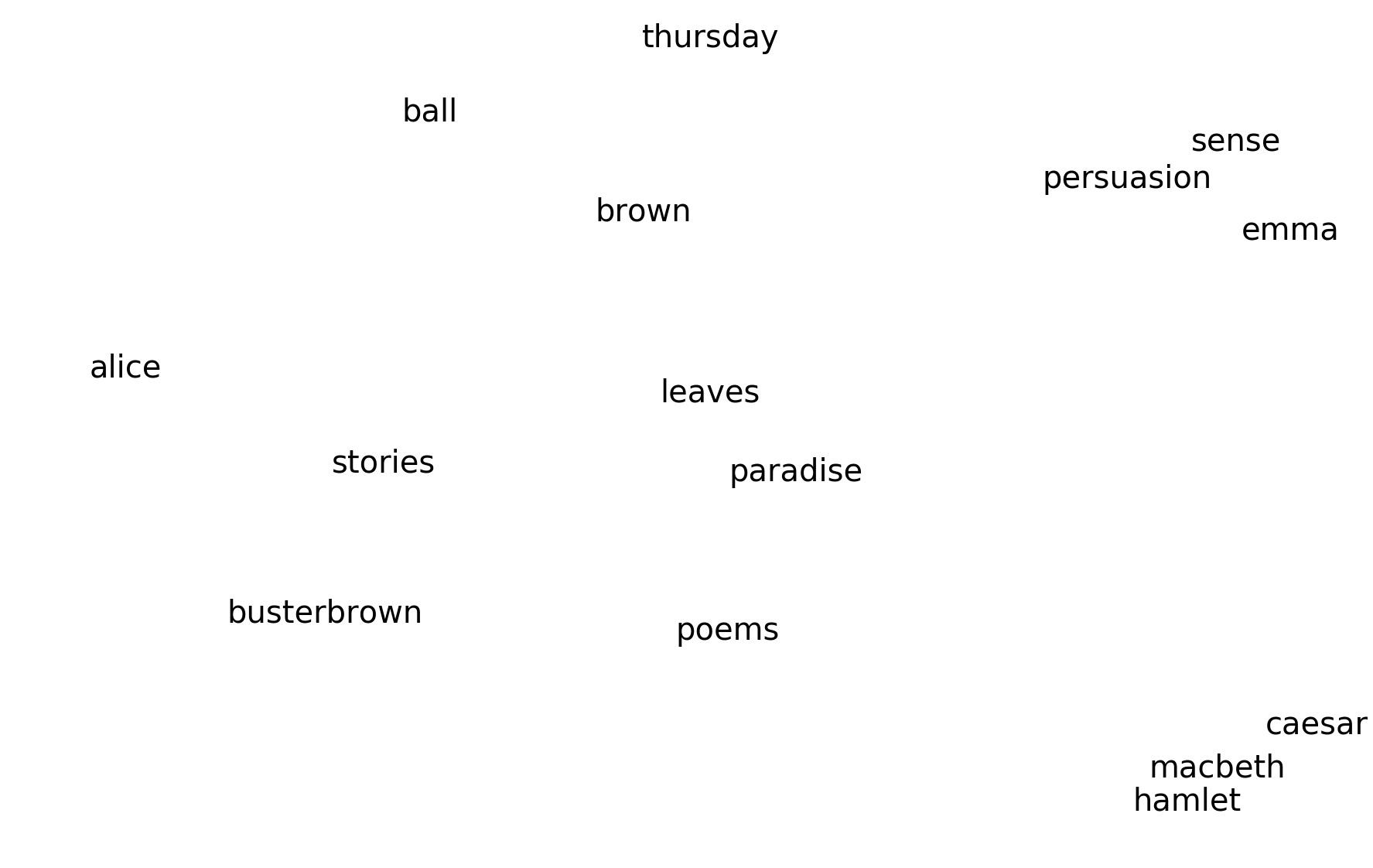
The sceptic in me reminds that t-SNE can sometimes suggest structure which isn’t really in the data. Still, these are some pretty dramatic clusters and with supporting evidence from k-means, we can pretty confidently declare that what we’re seeing is not an accident.

Epilogue

I guess the main lesson here is that simple techniques can get you pretty far. Tf-idf is basically just counting words and yet it told us quite a bit about our little dataset. Moreover, all the stuff we used is several decades old (except for t-SNE), so you don’t need the state-of-the-art to have fun with data. As for further steps, it would be tempting to repeat this analysis on a larger corpus and perhaps use it to train a classifier, but considering this post took me literally nine months to finish, I’m not promising anything.

Footnotes